
Guide
Reading your risk-adjusted schedule.
What the bars, tails, and percentiles actually mean, why tails land where they do, and the weekly loop that keeps the forecast honest.
1. Getting started
Five steps from a blank workbook to a risk-adjusted Gantt. The same list, plus system requirements, lives on Support.
- Install the Epoch SRA add-in: in Excel, Insert > Get Add-ins (or Home > Add-ins), search for “Epoch SRA” and click Add. Then click the Epoch SRA button that appears on the Home tab to open the task pane. In some organizations the add-in store is switched off by IT policy: if Get Add-ins is missing, greyed out, or the search will not install anything, ask your IT admin to allow Office Store add-ins for your account, or to deploy Epoch SRA centrally from the Microsoft 365 admin center (Integrated apps).
- Click Insert blank template to create the three empty structures: the
ESRA_Scheduletable (with theESRA_ProjectStartcell), theESRA_Risksregister, and theESRA_Eventslog. Your real data is kept untouched, and sample rows from See an example are treated as disposable and replaced, so the button is always safe to press. Have an MS Project schedule instead? Export it as XML (File > Save As > type: XML) and click Import MS Project XML. The file is never modified, and the import creates the empty register and event log alongside the schedule. - Fill the schedule (dates first; see below) and type your risks into the
ESRA_Riskssheet. The category and status columns carry in-cell dropdowns, likelihood and severity accept whole numbers 1–5, and the register section documents every column. Have an existing register elsewhere? Select its rows including headers and click Import from selected range: any layout works, columns are recognized by name and synonyms, and your cells are never modified. - Click Compute to run the analysis and write the
ESRA_Resultssheet, then Open full Gantt to see the risk-adjusted schedule (and Save as PNG to export it). - Want to explore first instead? See an example inserts a fictional demo schedule and register – see a full analysis in three minutes on the demo program, then run your own. In a blank workbook the demo is fully computable; in a workbook that already has your data, the demo sheets go in side-by-side as view-only and the forecast keeps reading your structures – the status line names exactly what stays canonical. Looking at an example never touches your data.
Entering a schedule by hand: dates first
The ESRA_Schedule table takes dates as first-class input, because PMs think in dates: give each row a planned_start + planned_finish and the working-day duration is derived, or a planned_start + duration_days and the finish is derived. A bare duration_days still works and schedules purely from links, exactly as before. If dates and a duration are both given and disagree, the dates win and Compute says so in a schedule note. Nothing is silently picked; a planned_finish alone is an error naming the row. Dates on a non-working day snap forward to the next working day, with a note. Which days are working is the ESRA_Calendar sheet’s decision (v1.2.0): the blank template creates it with the Mon–Fri default, and you can edit the weekday pattern (e.g. Mon,Tue,Wed,Thu,Fri,Sat), the hours per day, and a list of exception dates (holidays, or extra working days). No sheet means Mon–Fri, exactly as before. And the model is the same one the MS Project import uses: a dated task holds its date; risk pushes it later only, through its links or its own risks, never earlier.
2. Importing from MS Project
Export your plan from MS Project as XML (File > Save As > type: XML), then click Import MS Project XML in the pane’s Schedule section. The file is read on your machine and never uploaded; your .xml is read-only and is not modified. The translated schedule lands on an add-in-owned Imported_Schedule sheet as the ESRA_Schedule table plus the ESRA_ProjectStart cell. Your own sheets are not touched.
The stored dates are the baseline
The import reproduces your plan as stored: each task carries its file’s own Start and Finish into planned_start / planned_finish, and Compute pins every dated task at its stored start. The deterministic schedule shows MS Project’s dates; manually scheduled or not, dates come from the file either way. Risk then pushes tasks later only: through a translated link from a risk-stretched predecessor, or through the task’s own risks. Nothing ever moves earlier than the plan you imported. (One convention note: planned_finish is written as the working-day instant after the stored finish day, the same point-in-time convention every Epoch SRA sheet and chart uses, so derived durations equal MS Project’s working-day spans.)
The file’s calendar is the truth (v1.2.0)
The import reads your file’s project calendar – its working weekdays (Mon–Fri, 6-day, 7-day, whatever the file defines), its day length, and its exceptions (holidays and extra working days) within the schedule’s span – and writes it to the ESRA_Calendar sheet. That calendar then drives everything downstream: duration counting, lag conversion, the dates every offset maps to, and what “per week” means in the delay price. Same doctrine as stored dates: the file wins, and a re-import overwrites the calendar sheet. One visible consequence: the old “stored date falls on a weekend” warnings mostly dissolve – a date is flagged only when it is non-working under the file’s own calendar, which is a genuine anomaly worth reading; that rare case still snaps forward, reported as before. The report states what arithmetic you are getting: “Calendar: Standard – 5 working days/week, 8 h/day, 11 exceptions in range.”
Honest scope: the project calendar is simulated. Per-task and per-resource calendar assignments in the file are not – each is reported by name (“T014 uses calendar ‘Night Shift’ – simulated on the project calendar”), and extra base calendars are listed as present-but-unused, the same refuse-and-report contract as everything else.
What translates
- Tasks with their stored dates: each becomes a row, numbered
T001upward, scheduled from its stored Start/Finish. A task with no stored dates falls back to its work-hours duration, and is listed. Blank/null rows are skipped with a count. - All four link types – FS, SS, FF, SF – with their lags (v1.0.5.0): each becomes a typed
depends_onentry such asT003:SS:2. Lags are converted to working days using the file’s own working calendar, and leads (negative lags) translate too. Under the stored-date baseline every link is push-later-only: it can hold a task at or push it past its stored date, never pull it earlier. - Links touching summary rows are re-anchored to leaf level rather than dropped: a summary predecessor re-anchors to its last-finishing leaf descendant, a link into a summary to its earliest-starting leaf. Nested summaries resolve to leaf level; ties break to the lowest UID. Every re-anchoring is listed by name in the report.
- Milestones, from MS Project’s milestone flag, pinned at their stored date.
- Project start = the earliest stored task start, into
ESRA_ProjectStart. The file’s project-level StartDate is not used for scheduling; when the two disagree, the report shows both and says which was used.
What doesn’t translate
Two lag flavours have no exact working-day equivalent, and are refused by name rather than approximated: percent lags (they scale with the predecessor’s duration) and elapsed-time lags (calendar time that may span weekends). The same goes for a predecessor that doesn’t resolve (a task that isn’t in the file). Non-ASAP constraints (Start No Earlier Than and friends) are report-only: with the stored-date baseline a constrained task already sits at its stored date, so the report simply names each one. If a duration can’t be parsed it is written as 0 and named; if a task has a blank name it is named too, because the schedule reader requires one.
This is deliberate. Converting an elapsed lag to a fixed working-day lag would move dates by an amount nobody asked for, and you would have no way of knowing it happened. A named refusal is recoverable; a silent guess is not.
What the report’s counts mean
- tasks converted
- Rows written to
ESRA_Schedule, and how many are milestones. - rows skipped
- Summary/rollup rows (their children carry the work) and blank/null rows. Counted, never silent.
- links translated
- A per-type count line – FS, SS, FF, SF, and how many carry a lag – over every link that made it into
depends_on. - re-anchored
- Links whose summary endpoint was re-anchored to a leaf descendant and then translated. Each is named, with the leaf it now holds at. Resolved + re-anchored + not-translated + unresolved (+ any dropped from an empty summary) accounts for every link in the file.
- manually scheduled
- Informational only: how many tasks MS Project marks manually scheduled, counted over every row including summaries, the same numbers MS Project itself shows. Dates come from the file either way, so this is context, not an alarm.
- links not translated
- The remaining refusals – percent lags, elapsed-time lags, unknown type codes – listed individually with the reason, plus any predecessor that wouldn’t resolve. Each one is a dependency MS Project has and Epoch SRA does not.
What to do about a link that didn’t translate
Two honest options, and the report gives you the task ids for both.
Add the dependency by hand. In the ESRA_Schedule table, put the predecessor into the task’s depends_on cell. The column takes typed links – T003:SS, or T003:FS:5 for a five-day lag – so a refused link can be re-expressed exactly: decide what a percent or elapsed lag really means in working days on your program, and write that. This is the option that keeps your network intact.
Or accept the task as unlinked, but know what you are accepting. A task with nothing in depends_on cannot receive risk from upstream: its dates hold at the imported baseline unless its own risks fire. It will show a clean, flat bar and no tail, which reads as safety and is not. When a significant share of tasks are unlinked, the results header says exactly this, in one line.
3. How to read the Gantt
Every row is one task from your schedule table. The bar is your plan; the amber is what the simulation adds to it.
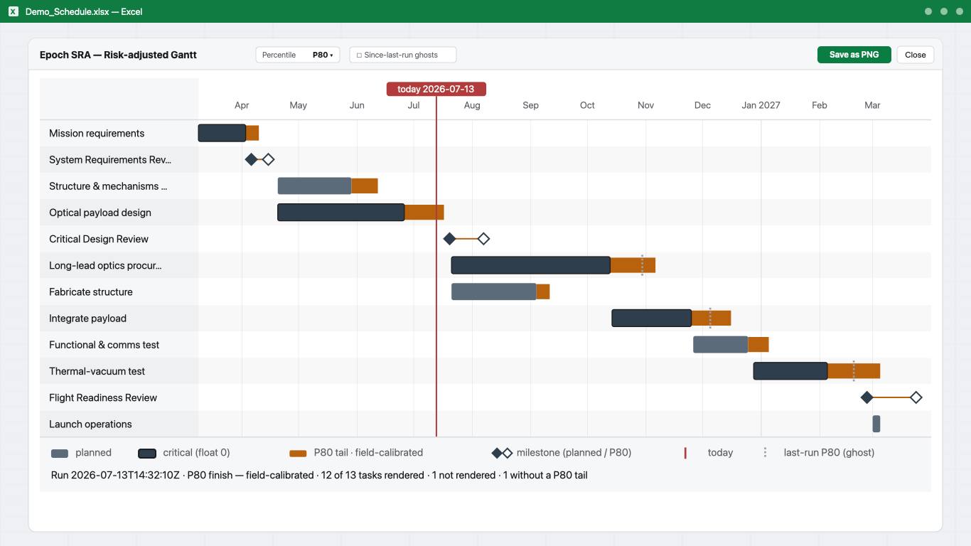
- planned
- The bar:
planned_starttoplanned_finish, straight from your table. Epoch SRA never moves it. - critical (float 0)
- A darker bar with an outline, so it survives greyscale printing. It reads the
is_criticalcolumn ofESRA_Results, which the engine sets when total float is zero within a rounding epsilon. - P80 tail · field-calibrated
- The amber extension, from the planned finish to the selected percentile’s finish. Its length is the schedule exposure: how much later than plan the simulation puts this task. The second half of the label is the provenance of the percentile you selected, not a fixed string.
- milestone (planned / P80)
- Milestones draw no bar. They draw two diamonds joined by a connector. Solid is the planned date, hollow is the selected percentile’s date. The gap between them is the slip. The hollow diamond only appears when there is a tail.
- today
- A vertical line with an ISO-dated chip. It is drawn only when today falls inside the chart’s date range, so it is absent on a purely historical or future window.
- last-run P80 (ghost)
- A dashed vertical line per row marking where the previous Compute put that task’s P80 finish. Toggle it with Since-last-run ghosts; the checkbox is disabled when there is no prior run. Ghosts always mean P80, whichever percentile you are viewing.
The line under the chart
It reads something like Run 2026-07-13T14:32:10Z · P80 finish – field-calibrated · 12 of 13 tasks rendered · 1 not rendered · 1 without a P80 tail, and it is stamped into the frame itself so an exported PNG can never lose its provenance.
Not rendered and without a tail are different failures. A row is not rendered when it could not be drawn at all (a missing or unparseable planned_start, a finish before its start, a year outside 1990–2100), and it carries the reason. Rendered plus not-rendered always equals the number of rows in the sheet; a row is never silently dropped. A row without a tail was drawn normally and simply had no exposure to show.
4. The charts
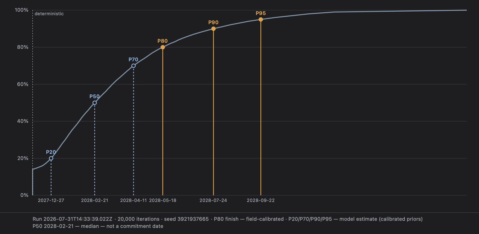
After Compute, Open charts gives you four views of the same run. Each carries its run timestamp, seed, iteration count and percentile tiers inside the image, so a chart pasted into a review deck cannot lose the context it was computed under. Save as PNG exports at 2×.
S-curve
Cumulative confidence against finish date: for any date, the share of simulated runs that finished by it. The markers follow one colour law throughout: amber is a commitment (P80 and above), and a cool dashed marker is a reference you should not commit to (P20, P50, P70). The dotted line is the deterministic finish: where the plan lands with no risk at all.
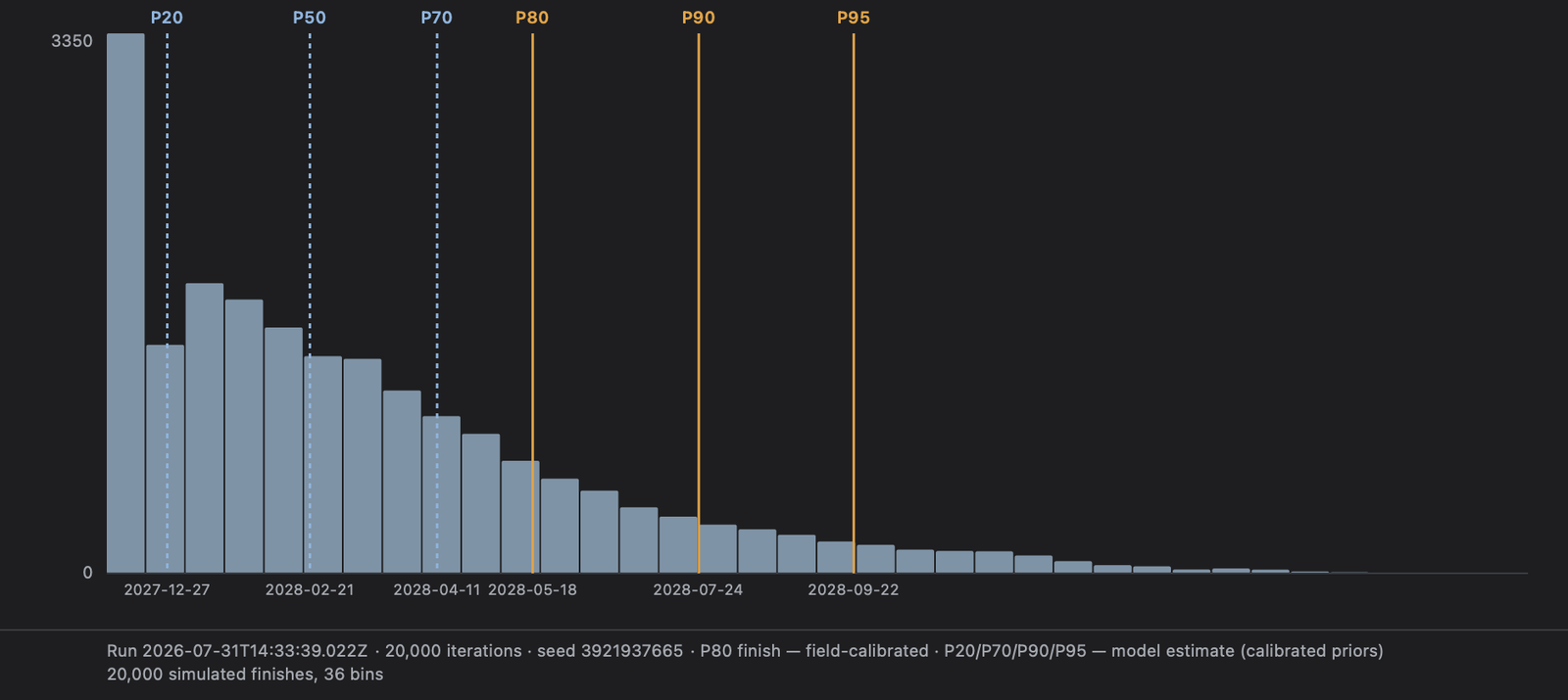
Histogram
The same run as a distribution: every simulated finish, binned. It shows the shape the S-curve smooths away: whether the spread is tight or long-tailed, and whether it is lumpy.
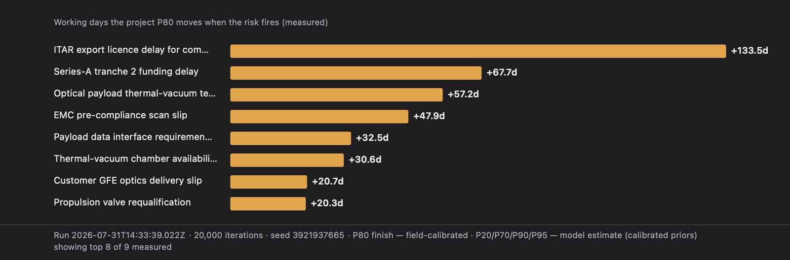
Tornado: measured, not estimated
One bar per risk: the working days the project P80 moves between the runs where that risk fired and the runs where it did not. It is measured on the run's own samples, not calculated from probability × impact beforehand.
This matters when you compare tools. The task pane's top risk drivers list ranks by an up-front estimate; the tornado ranks by observed effect. They will not always agree, and that is correct. An up-front estimate cannot know that a risk lands on a path that was already late, or that two risks bite the same slack. Where they disagree, the tornado is the one that watched what happened.
A risk that never fired, or is certain to fire, has no two worlds to compare, so it has no bar; it is counted as not measurable this run rather than shown as zero. A bar from very few firings is marked thin. The footer states how many risks were measured and how many bars are shown, so a truncated list never reads as the whole list.
Sensitivity
One row per task, sortable by either column.
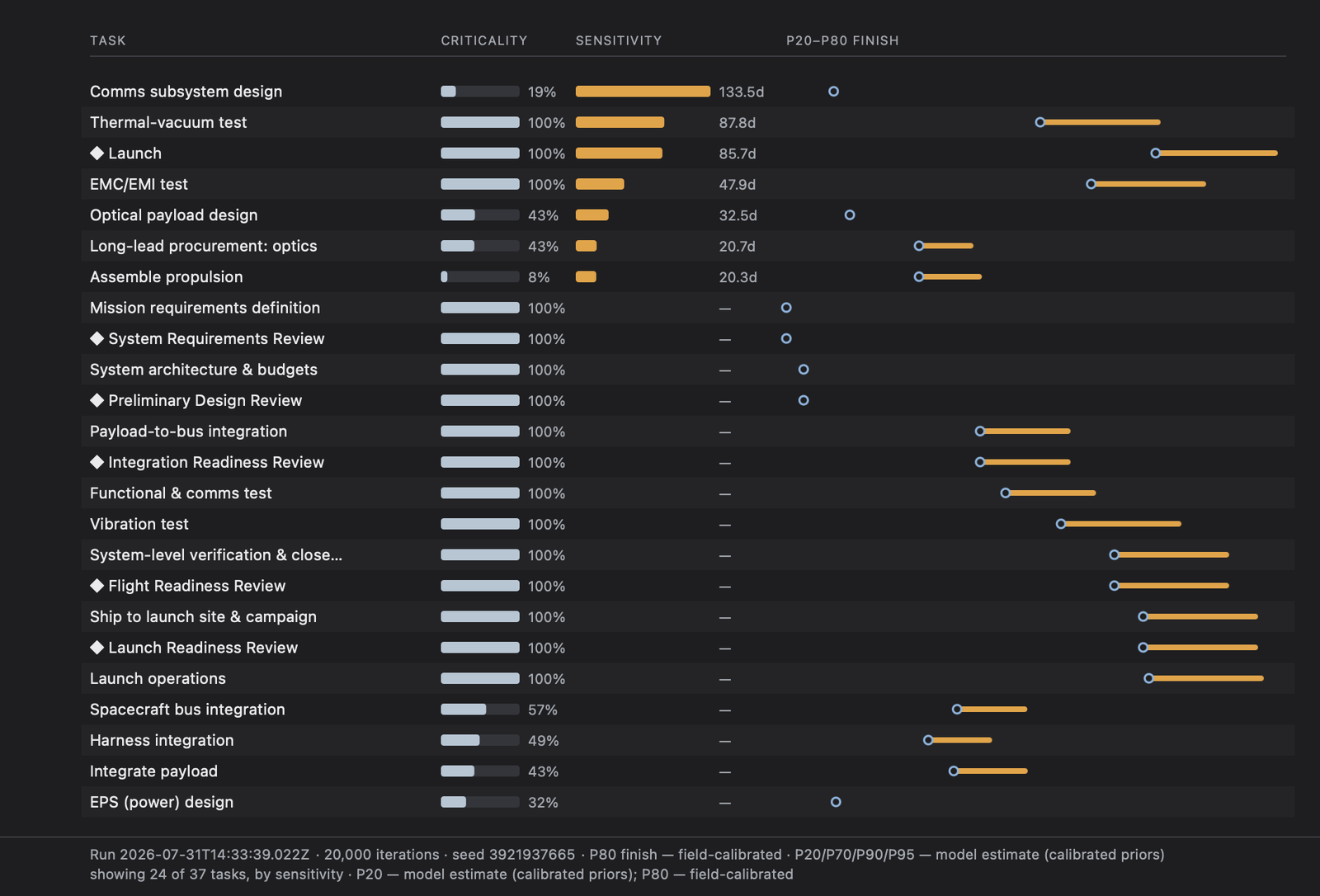
– in sensitivity means no mapped risk, not zero effect.- criticality
- The share of iterations the task landed on the critical path. 100% means it was always critical; a task at 40% is only sometimes the thing holding the date.
- sensitivity
- The measured contribution of the risks mapped to this task: how much the project P80 moves because of them. A task with no mapped risk shows
–. - P20–P80 finish
- When this task finishes, across the run. The low end is a reference dot, the amber bar runs to the P80. All rows share one date scale, so the bars are comparable.
The two numeric columns answer different questions and are worth reading together: sensitivity is measured against the project finish, criticality is about this task. A task can sit at 19% criticality and still be the largest single contributor to your P80: rarely on the critical path, yet carrying the risk that moves the program when it bites. Sorting by criticality alone would bury it.
Where P20 comes from
P20, P70, P90 and P95 appear only when Extended percentiles is ticked before Compute, which also raises the run to 20,000 iterations, because deep quantiles are lumpy at 5,000. All four are labelled model estimate (calibrated priors): same simulation, same calibrated priors, but the field evidence is against P80, not against them.
P20 is written to ESRA_Results and shown in the charts, but the Gantt never offers it. That is deliberate. The Gantt's tail is drawn in the commitment colour, and P20 is an optimistic bound: an 80% chance of missing, not a planning date. An amber P20 tail would say “commit to the date you will almost certainly miss.”
5. Percentiles
The selector offers exactly those percentiles whose p*_finish column exists in ESRA_Results. By default that is P50 and P80. It opens on P80 and never auto-selects P50.
P50: the median, not a commitment
Half the simulated outcomes finish later than this date. That is the whole meaning of it. The Gantt labels it P50 (median – not a commitment date) and the status line spells out the consequence: P50 finish (median – 50% chance of missing). It is deliberately drawn in a cool outline rather than the amber commitment styling, because a median presented in commitment colours is a date someone will quote in a review. Useful as a reference: if your plan sits far from P50, the plan is optimistic before any risk is considered.
P80: field-calibrated, the level to commit to
Four runs in five finish by this date. This is the default view and the one the product is built around: P50 and P80 are field-calibrated against replayed historical programs, which is why the legend says field-calibrated rather than a bare “calibrated”. When you are asked for a date to defend, this is the one that has been checked against what actually happened on real programs.
P70 / P90 / P95: model estimates, stress views
These are off by default. Tick Extended percentiles (P70 / P90 / P95) in ESRA_Results before you Compute, or the columns are never written and the selector will not offer them. They are labelled model estimate (calibrated priors), truncated to model estimate in the tight legend, and the distinction is deliberate. They come from the same simulation on the same calibrated priors, but the deep tail depends on distribution shape and risk correlation that the field evidence does not yet pin down. Read them as stress views: what a bad run looks like. Do not read them as a calibrated commitment, and do not quote P95 as a date.
6. Why tails appear where they do
A task with no mapped risk still has a tail.
Correct, and it should. A task’s percentile finish comes from the simulated network, not from the risks mapped to that row. If a predecessor’s distribution pushes its finish later, everything downstream inherits the shift through its dependencies. A tail on an unmapped task means its predecessors are uncertain: it is exposed, not risky. To shorten it, look upstream.
At P50, almost nothing has a tail.
Expected. A tail is drawn only when the selected percentile’s finish is later than the planned finish; equal or earlier draws nothing, and the row is counted in the footer as without a P50 tail. P50 is the median, so for much of the network the median outcome lands on or before the plan. That is the 50% frontier, not a missing calculation. It is also the point: at P50 the schedule looks fine, which is exactly why committing to it is a coin flip. Switch to P80 to see the exposure.
Some tasks show no tail, and the status says unlinked.
An unlinked task names nothing in depends_on: it sits in the sheet without sitting in the network. Compute says so plainly: unlinked tasks (2): T07, T09 – dates without depends_on receive no upstream risk. Nothing upstream can reach it, so it shows no tail however risky its predecessors are; it hasn’t got any. It is not a safe task, it is an unmodelled one, and the flat bar is the tool telling you it has nothing to say about that row.
Two things cause it. Either the task’s dates came from a planned_start/planned_finish pair and no dependency was ever given; or it arrived from an MS Project import whose links didn’t translate. An SS link or a lagged link is reported, not converted, so the task lands with an empty depends_on. Check the import report against this list. The fix either way: give it a predecessor in depends_on (typed links are allowed, e.g. T003:SS), or map a risk directly to it.
The last milestone’s tail is huge.
It accumulates, and two things concentrate there. First, propagation: every upstream distribution feeds the terminal milestone through the dependency chain, so its spread is the network’s, not one task’s. Second, scope: a risk marked PROGRAM_WIDE, or left with no mapped tasks at all, resolves onto the terminal sink: the no-successor task whose early finish is the project finish. It lands squarely on your last milestone. Before you argue with the arithmetic, check how many of your risks are program-wide.
7. The Tuesday loop
The schedule stays current because you tell it what happened, not because it guesses. The loop is: log what happened, Compute, read what moved.
Log an event
An event is something that has happened, as opposed to a risk that might. Type it as a row in the ESRA_Events sheet: an event_id (E01 style), a title describing what happened, the date it became known (yyyy-mm-dd), a category from the in-cell dropdown (use other when none fit), the affected_tasks, and magnitude_days: your best believed estimate of the damage in working days. The pane's Events list names each row and follows the sheet.
Nothing moves yet. The event carries a not yet computed marker until you click Compute. Written to the sheet is not the same as folded into the forecast. Scope works like the register: write PROGRAM_WIDE in affected_tasks to land the event on the terminal milestone, or leave it empty to keep it a draft; a draft is explicitly not applied until you fill in tasks. Converted risks arrive here automatically, carrying the source risk's title.
Record the actual
When the damage is known, the event sits under Awaiting actuals with an actual (wd): field and a record button. Record it and the row reads believed 15 → actual 20 wd on T03. (Forecast still uses believed.)
That parenthesis is the important part, and it is not a limitation. The forecast is mutated by the believed magnitude and never by the actual. If a recorded actual retroactively rewrote the forecast, every past run would silently improve itself with information it did not have at the time, and you could never reconstruct what the tool told you in March. No look-ahead, so the run you defended in a review still says what it said.
What SINCE LAST RUN shows
It compares your previous Compute with this one: the project finish and every milestone’s P50 and P80, plus events added, removed, or changed in magnitude, measured in working days from each run’s own start, so a rebased project start does not fake a movement. On a first run it says so: First run – nothing to compare yet. When something moves, it attributes it: Event E3: supplier slip +15d on T13 → finish P80 +11d. The Gantt ghosts read the same snapshot.
What recording actuals does (and does not) do
It builds the believed-versus-actual record in your workbook. That record is what makes the priors improvable: it is the evidence of how far off the estimates were, per category, on a real program.
It does not re-fit anything on your machine. The add-in never edits its own priors, and nothing you record changes your numbers. Priors move only when a new domain pack ships, after that evidence has been replayed against the backtest programs. This is a deliberate line: a tool that quietly re-tunes its model under a live program produces forecasts nobody can reproduce or audit.
8. Register basics
The sheet is the register
The register is yours: no import path ever writes or clears it, and you author it directly in the ESRA_Risks sheet. Clicking a risk in the pane's list selects its row; the pane shows status, the cells hold the data. One rule set validates every row however it arrived: typed, imported, or sample.
The columns
- risk_id
- Your identifier, unique per row. R01 style keeps sorting sane, but any non-empty id works.
- title
- What the risk is, in your words. This is the name the pane and reports use.
- category
- Yours. Free text, optional, never validated: your program’s own taxonomy (“Payload thermal”, “Customer ICD churn”), preserved verbatim through import, merge, and re-import. It is display, sort, and report metadata – it never touches the statistics.
- prior_class
- The statistics. One of the eight calibrated ids from the in-cell dropdown – pick the nearest failure pattern; the table below is the reference. This is what prices the risk: impact priors are calibrated per prior_class. A risk with a blank prior_class is not overlaid, and Compute says so by name (“N need a prior_class”) rather than guessing. Event-only ids are rejected here.
- likelihood, severity
- Whole numbers 1–5 (ECSS 5×5). The cells reject anything else.
- risk_index
- Derived, never typed: the sheet holds a live =L×S formula and the ECSS heat-map.
- affected_tasks
- Comma-separated task ids from
ESRA_Schedule(for exampleT001, T004), the single wordPROGRAM_WIDE, or empty (unmapped; see the scopes below). - status
- One of
open / closed / realized / retired / removed, from the dropdown. Blank reads as open. - owner, notes
- Free text. Notes feed the mapping suggestions’ keyword matching.
- distribution
- Optional override. Blank on every row by default, and blank means the reference triangular prior – leave it alone and nothing changes. Set it from the dropdown to read the same min/most-likely/max through another shape; the profile panel then shows Source: you. See Choosing a distribution.
prior_class reference
Your categories are yours; prior_class picks the statistics. Cells store the bare id; this table is what each one means. Risk-capable ids (usable in the register): supplier_slip supplier delivery slip · test_failure test failure and retest · requirement_change requirement change · export_control_delay export control / licensing delay · lli_delay long-lead item delay · customer_delay customer-side delay (GFE, reviews) · funding_event funding event (payment or round delay) · ncr_waiver non-conformance / waiver. Event-only ids (valid in ESRA_Events, rejected in the register): launch_manifest_change launch manifest change · key_person_loss key person loss · team_resize team resize / re-allocation · wp_restructure work package restructure. Events additionally accept other for anything outside the taxonomy.
Registers created before the split (a single category column) keep working: on read, a category value that matches a calibrated id is used as the prior_class – your original value stays in category untouched – and the migration is reported in the pane. The sheet gains the prior_class column on its next register write (an import or a re-insert).
L × S scoring
The register is ECSS-M-ST-80 5×5: likelihood and severity, each 1–5, and risk_index = likelihood × severity, 1–25. Two details matter in practice. The index is written into your sheet as a live formula (=E2*F2) rather than a number, so it cannot go stale the moment someone edits L or S; and the add-in derives it on read regardless, ignoring whatever the column holds.
The red/amber/green colouring is not a threshold on the index. It is an explicit 5×5 lookup, and it is asymmetric on purpose: high severity turns red sooner than high likelihood does. A 4×2 and a 2×4 both index 8 and do not get the same colour. Do not infer a band from the number.
Importing a register that scores in words works: High maps to 4, Very low to 1, and so on, and the mapping is noted per cell. Values above the scale are clamped to 5.
Mapped, program-wide, unmapped
There are three scopes, not two, and the third is a question rather than an answer.
- mapped
affected_tasksnames real tasks. The risk overlays those rows.- program-wide
- The literal
PROGRAM_WIDEtoken: a decision that the risk bites the whole program. It overlays the terminal sink. - unmapped
affected_tasksis empty. This is an undecided risk, not a program-wide one. It still overlays the terminal sink so it is never silently ignored, but the accounting counts it separately: an empty cell is a question you have not answered yet.
Suggest mappings proposes risk-to-task links from deterministic keyword overlap, for open risks only. Since the category split it also proposes a prior_class for risks that lack one, from your own category wording. Every suggestion – task or prior_class – is a proposal you accept or reject; it never auto-links and never auto-sets. It will sometimes be confidently wrong (a construction-noise risk whose keyword “vibration” hooks the vibration test), which is why it asks.
What overlays, and what does not
Only open risks overlay. A closed, realized, or retired risk is a real outcome and is excluded; a risk with a linked_event has become an event and is counted there instead, never twice. Two categories, supplier slip and long-lead-item delay, are skipped with a stated reason rather than a silent zero: they price from a reported slip duration, which a 5×5 row does not carry. If nothing overlays, the pane says so plainly rather than showing you an unadjusted schedule that looks computed.
Merge or replace on re-import
An imported register’s category column arrives verbatim into category – whatever taxonomy your program uses is kept, not translated. prior_class starts blank on newly imported risks and is reported (“N risks need a prior_class before compute”); a prior_class you have already confirmed survives every re-import that does not explicitly carry one.
Re-import is refreshable and non-destructive. Merge (the default) updates matching risks and keeps the rest, preserving your task mappings: a re-import does not undo an afternoon of mapping work. Replace marks open risks that are absent from the source as withdrawn, with the reason recorded.
Neither mode deletes a row, and your source range is never modified; the importer only reads it. A withdrawn risk that reappears in a later import is re-opened by that evidence.
9. Choosing a distribution
Every risk is priced from its prior_class: a min, a most-likely and a max, calibrated per failure pattern, then scaled by your severity score. Those three numbers can be read through more than one shape, and the optional distribution column on ESRA_Risks lets you say which. Leave it blank – as every risk is by default – and nothing changes: the calibrated triangular is used, and the column may as well not exist.
Choosing a shape does not ask you for new numbers. All four families read the same min/most-likely/max the prior already supplies; you are choosing how the mass between them is distributed, not re-estimating the risk.
- Triangular (calibrated default)
- Straight lines from min up to the most likely and down to max. This is the shape the priors were calibrated as, so it is the only one whose output carries the field-calibrated claim. Use it unless you have a specific reason not to – and if you are unsure, that is a reason to stay here.
- PERT
- A smooth curve over the same range, weighted toward the most likely value. Same bounds as the triangular but less mass out at the extremes, so it produces a slightly tighter band. Use it when the most-likely value is genuinely the best information you have and the min/max are more like outer limits than live possibilities.
- Lognormal (bell shape, floored at zero)
- A rounded, right-skewed curve with a hard floor at zero and no upper bound. The most likely value is honoured exactly and your max is placed at the 90th percentile – so roughly one draw in ten lands beyond it, which is the point: use this when the risk has a genuine tail and “max” is your realistic bad case rather than a wall. Note the trade: your
minis not used. For a lognormal with a fixed mode there is generally no shape that also puts the 10th percentile at your min, so the fit honours the mode and the upper tail, and the pane says so rather than pretending otherwise. - Uniform (flat, ignores most likely)
- Equal probability everywhere between min and max. It reads only min and max – your most-likely value is discarded, and the pane and the report both say which value went unused. Use it when you honestly have no idea where within the range the answer sits; it is the widest of the four and will usually give the latest P80.
Why there is no normal option
A normal distribution is symmetric and unbounded, so it places real probability below zero: a risk that fires and makes the project finish earlier. Truncating it at zero is not a fix, because clipping the tail shifts the mean and every percentile away from the parameters you were shown – the tool would display one distribution and simulate another. And being symmetric, it cannot represent a three-point estimate whose most-likely value sits off-centre, which is every prior in the pack. If you are looking for a bell, Lognormal is the one to pick.
Typing anything else into the cell is refused by name, with the four legal values listed – a typo never silently falls back to the default.
Where a shape comes from
Every parameter is described by where it came from, never by what it lacks. Leave the column blank and the shape is Epoch reference data; choose one and it is yours. The profile panel says which, in one neutral line – Source: you or Source: Epoch reference data – and it appears in the panel only, never as a badge in the register list and never in a warning colour. The register row shows the family name alone (pert) when you have chosen one that differs from the reference default; an explicit triangular is the default written down, so it shows nothing at all. ESRA_Results and the report’s risk-assumptions table name the family and who chose it, factually.
The shape preview
Selecting a risk in the pane shows a small sparkline of the distribution it actually samples, with ticks at min, most likely and max. It is drawn from the engine’s own sampler rather than a decorative curve, so switching family redraws it because the sampled distribution changed – what you see is what runs. The same preview appears per row in the report’s risk-assumptions table. A lognormal’s curve is clipped on the right with a note that the tail continues; there is no combined overlay of several risks, because risks on shared axes invite comparing areas that are not comparable.
Where the choice lives
In the sheet, like everything else: the distribution cell is the single source of truth, and the pane selector is an editor for it. The choice survives re-import (a refresh updates the source’s facts, never your modelling decisions), is recorded in saved scenarios, and shows up in the delta view when you change it – “R01 distribution changed triangular → lognormal” – so a moved forecast is never unexplained.
10. Cost (v1.1.0)
Cost is optional and off by default: leave the cost columns blank and nothing cost-related appears anywhere – that sentence is the only pointer you will get. Fill them in and the same simulation that prices your dates also prices your money: no new sampling, no separate model, and your schedule results are bit-identical with or without cost inputs.
The columns
- cost_per_day
- On
ESRA_Schedule. A burn rate in workbook currency per working day of the task’s simulated duration – a working day as the schedule’s calendar defines it (the imported file’s calendar, orESRA_Calendar; see the import section). When a risk stretches the task in an iteration, that iteration’s cost grows by the rate times the added days. Blank = 0; non-negative numbers only. - fixed_cost
- On
ESRA_Schedule. Money incurred once when the task runs, independent of duration. Every task in the network runs, so this lands in every iteration and in the deterministic baseline. Blank = 0. - cost_impact
- On
ESRA_Risks. Money added in any iteration where the risk fires, alongside its schedule impact – the same coin flip decides both, so the two can never disagree. Blank = 0. A risk that is skipped at compute (no prior_class, wrong status) contributes no cost either: it is reported, not silently priced.
The blank template carries both schedule cost columns. On a schedule imported from MS Project XML you can add them by hand – but note that re-importing the XML rebuilds the table and the typed rates do not survive; carrying them through re-import is on the R2 list.
Currency
One workbook-level setting in the pane (default EUR), used to label cost outputs. Display only: no conversion, no FX – the numbers are whatever currency your rates are in.
What you get, and what it is
The results sheet and the pane gain a cost block – deterministic cost, cost P50 and P80 (the extended toggle adds the deep set) – and the charts gain a cost histogram and a cost measure on the tornado, so you can rank risks by the money they move, not only the days. The delay price is the expected cost per week of finish slip past P50, measured as the slope of cost against finish across the run’s simulated futures at your rates – the line always states that basis.
Provenance, stated once and printed everywhere: cost numbers are derived from the calibrated schedule simulation through your rates – rates are yours, distributions are the schedule’s. Cost percentiles are never labelled field-calibrated: the backtest campaign validated P80 dates, and that claim does not extend to money.
11. Licensing
The 7-day trial needs nothing: no signup, no card, no key – it starts on your first Compute. A purchased license key (ESRA1.…) is pasted into the pane’s License section. Applying a key activates it for that machine with one connection, once; a key activates on up to its purchased number of seats, and re-activating the same install (a reinstall) does not use another seat. What activation sends and stores is stated in the pane at the moment it happens and in the privacy policy: the key id, a random install identifier, the optional machine label, and the date.
Deactivating a machine
Retiring a laptop? Deactivate this machine in the License section frees its seat so the key can activate elsewhere. Reassignment and deactivation requests by email are honoured from the purchasing contact or an address at the purchasing organization’s domain.
Offline activation
On a machine without a connection, the pane offers offline activation when the online attempt fails: it shows a short request code (ESRA-REQ1.…). Email that code to sales@epochsra.com from your purchasing contact; you receive an activation token (ESRA-ACT1.…) to paste into the same panel. The token is verified on the machine itself, and the install behaves exactly like an online-activated one from then on.
How the numbers were measured (calibration-v1)
Most schedule risk tools ask you to trust textbook distributions. We didn’t think you should have to – so we tested ours against programs we had lived through.
We took completed space programs – the schedule as it was planned, the risk register as it was kept, the events as they actually hit – and replayed each one through the engine as if the program were still live. Then we graded our own forecasts, milestone by milestone, against the dates each program actually delivered. Before grading anything, we audited every history against the program’s recorded dates and outcomes – every figure in the record is checked against what really happened, not against anyone’s impression of it.
We let a risk category earn the field-calibrated label only the hard way: a risk of that kind actually fired on a real program, and our prior proved consistent with the impact that followed. Where a category is still waiting for that evidence, we carry it as a structured estimate, with its reason recorded. And every output labels which tier its numbers stand on, per item – you always know whether a figure was checked against the field or derived from the same calibrated machinery.
We closed the campaign as a dated, change-controlled record: calibration-v1. If we ever change a prior, we owe a full rerun of the calibration matrix and a recorded before/after. The numbers cannot drift quietly – and neither can we.
The full record – the per-program matrix, the residual ledger, and the rules that govern future changes – lives in our change-controlled decisions log.
12. Glossary
P50 and P80 dates
A P-value date is a confidence level over simulated outcomes: the P50 date is the median (half the simulated runs finish later), and the P80 date is the date 80% of runs finish on or before. In Epoch SRA, P80 is the commitment level and is field-calibrated against replayed historical program actuals; P50 is drawn as a cool reference, never in commitment styling, because committing to a median is a coin flip.
Merge bias
Merge bias is the systematic lateness that appears where parallel paths merge: the merge point must wait for the slowest incoming path in every simulated outcome, so its expected date is later than any single path suggests. Deterministic CPM schedules cannot show this effect; Monte Carlo simulation reproduces it naturally, which is a large part of why simulated dates sit to the right of the plan.
DCMA 14-Point Assessment
The DCMA 14-Point Assessment is a schedule-quality checklist published by the US Defense Contract Management Agency, covering structural health measures such as missing logic, leads and lags, relationship types, constraints, float, and baseline execution. It scores whether a schedule is well-formed enough to analyze – it is a format for schedule hygiene, not a simulation method, and it is widely used as the common vocabulary for schedule health across defense and space programs.
GAO Schedule Assessment Guide
The GAO Schedule Assessment Guide (GAO-16-89G) is the US Government Accountability Office’s reference on what makes a project schedule reliable, organized around ten best practices – among them capturing all activities, sequencing with valid logic, establishing durations and float honestly, and conducting a schedule risk analysis. It is guidance for building and auditing schedules, not a scoring tool; auditors and program offices use it as the standard of care a schedule is judged against.
NASA Schedule Management Handbook
The NASA Schedule Management Handbook (NASA/SP-2010-3403) is NASA’s agency-level guidance on planning, building, statusing, and assessing program schedules, including schedule health assessment practices and the use of schedule risk analysis on flight programs. Like the GAO guide, it describes practices – it does not review or approve tools; it is the schedule-management reference most space programs already work to.
Schedule quality diagnostics
The checks a tool runs on the network before it trusts a simulation of it, on the principle that an analysis is only as good as the network under it. Epoch SRA’s checks are aligned with the DCMA 14-Point Assessment (8 of the 14 points implemented, listed below) and informed by the GAO Schedule Assessment Guide and NASA Schedule Management Handbook practices – aligned with and informed by, no more: no agency has reviewed or approved Epoch SRA, and no such claim is made anywhere.
Every Compute runs the assessment and writes a Schedule quality (DCMA-style) section to the pane and to ESRA_Results. The eight implemented points, evaluated from schedule structure and the CPM pass:
- 1 – Logic
- Tasks missing a predecessor or successor (the project’s own start and finish are legitimately open); dangling tasks receive no upstream risk.
- 2 – Leads
- Negative lags on relationships – schedule compression that hides sequence risk.
- 3 – Lags
- Positive lags – waiting time encoded in links instead of visible tasks.
- 4 – Relationship types
- Share of links that are Finish-to-Start; heavy SS/FF use makes a network harder to reason about.
- 6 – High float
- Tasks with implausibly large total float – usually a sign of missing logic.
- 7 – Negative float
- Tasks already later than the schedule can absorb.
- 8 – High duration
- Tasks too long to status meaningfully – candidates for decomposition.
- 12 – Critical path test
- A perturbation test: stretch a critical task and confirm the finish moves – the network’s logic actually carries the critical path.
Not yet checked (each reports not applicable by name, never a silent pass): 5 hard constraints (needs constraint metadata), 9 invalid dates and 11 missed tasks and 14 Baseline Execution Index (need a status date, baseline, and progress), 13 Critical Path Length Index (needs a contract finish), and 10 resources (resource loading is out of scope by design). Refuse-and-report, applied to marketing.
Alongside the 14-point table, the shipped diagnostics remain refusals with names attached: the import report counts what was converted, skipped, re-anchored, or left manually scheduled, and names every link it could not translate with the reason; at compute, risks without a prior_class are counted by name, and a run in which no uncertainty took effect says so above the results rather than posing as a forecast.
Discrete risk vs duration uncertainty
Duration uncertainty is the spread around how long planned work takes; a discrete risk is an event that either happens or does not, adding its own impact when it fires. Epoch SRA models discrete risks from the register – each open risk overlays its mapped tasks with a calibrated, category-priced impact at its scored likelihood – and treats occurred events as deterministic schedule mutations, so a realized risk is converted and never double-counted.
ECSS-style 5×5
ECSS-M-ST-80 is the European space standard for project risk management. Its scoring convention is a 5×5 grid: likelihood 1–5 times severity 1–5, giving a risk index of 1–25 that is banded into green, yellow, and red. Epoch SRA’s register uses this convention – likelihood and severity are whole numbers 1–5, the risk_index is a live =L×S formula under the ECSS heat-map – and the scored likelihood and severity are what price a risk’s impact in the simulation.
GFE
Government-furnished (or customer-furnished) equipment: hardware, models, or facilities the customer contractually supplies to the program. A late GFE delivery is a classic customer-side schedule driver – the receiving team can be fully on plan and still slip. In Epoch SRA’s taxonomy, GFE deliveries fall under the customer-side delay category.
TVAC
Thermal-vacuum testing: a test campaign in a chamber that reproduces the thermal and vacuum environment of space. TVAC chambers are scarce, shared facilities, so slot availability and campaign re-runs are recurring schedule drivers on flight programs. In an Epoch SRA register, a failed TVAC campaign is a test failure and retest risk; a slipped chamber slot is typically logged under supplier or customer-side delay, depending on who provides the facility.
NCR / waiver
An NCR (non-conformance report) records that a produced item deviates from its specification; a waiver (or deviation) is the formal decision to accept and fly it as-is rather than rework it. The disposition loop – write-up, review board, decision – takes calendar time whichever way it goes. Epoch SRA carries non-conformance / waiver as its own risk category, so this loop can be priced instead of absorbed silently.